続・時系列予測をさらに究める。自己回帰モデルによるアプローチ(「IISIA技術ブログ」Vol. 14)
このブログにおける前回記事において、時系列予測について自己回帰モデルによるアプローチも弊研究所として試してみる価値はあるのではないかと言及した。今回はその続きであり、[Peixeiro 23]に基づき、実装したコードによる演算結果について考察を行う(したがってなぜこの実装及び検証が必要なのかは前回記事を読まないとお分かり頂けないと思うので、セットでお読み頂くことをお勧めする)。
コーディングは[Peixeiro 23]で掲載されているものを参考にしたが、そこで題材として取り上げられているデータは、米国における家庭の電力消費量を追跡するデータセット(Individual household electric power consumption)である。このデータセットはUCI Machine Learning Repositoryで公開されている。しかし今回、この実装・検証を行う理由は弊研究所がご提供している各種金融指数のヴォラティリティ分析ツールであるPrometheus I/IIを超えるモデルとして、果たして自己回帰モデルを採用すべきかどうか、確かめることにある。そのため、まずはデータセットについては[Peixeiro 23]の方針を変更し、典型的な金融指数に関する時系列データ(time-series data)を採用しなければならない。
そこで今回はStooqより日経平均株価データを取得し、実装することとした。また前処理について[Pexeiro 23]はデータラングリングとデータ前処理と称していくつかの手法を採用している。しかしこの部分についても、Prometheus I/IIとの比較を念頭に置きつつ、そこで採用しているのと同じ前処理の手法で処理し(この部分は営業秘密に該当するため、コードも含め詳細は割愛させて頂く)、最終的に訓練データ、検証データ、そしてテストデータの3つに分割することとした。
以上の前処理済みデータセットを実装する先として「ベースライン」「ARLSTM(自己回帰型LSTM)」及び「CNN+LSTM」の3つのモデルを用意した。まず「ベースライン」についてであるが、[Pexeiro 23]は1)時系列データの最後の既知の値を繰り返すもの、2)最後の24時間のデータを繰り返すもの、の2つを採用している。しかし今回は上述のとおり、我が国において毎営業日ごとに5時間のみ作動する「日経平均株価」の時系列データを採用するため、これら2つの内、1)のみを採用することとした。
「CNN+LSTM」については弊研究所のPrometheusシリーズにおいて採用しているアルゴリズムと原理的には同じであるものの、そこで実装されているモデル(コード)そのものではないことをここで明記させて頂く。あくまでも[Pexeiro 23]が提示しているコードを微修正する形で用い、「ベースライン」及び「ARLSTM」との比較を試みる。なお、[Pexeiro 23]ではIndividual household electric power consumptionデータセットに関する時系列分析に関する限り、「ARLSTM」が一番優れていると結論づけていることを合わせて明記しておきたい。
[Peixeiro 23]においてはIndivudual household electric power consumptionデータセットにつき、24時間分のデータを使って次の24時間を予測するというデータウィンドウ処理(data windowing)を採用している。しかしこの部分については日経平均株価の時系列データに関する上述の特徴上、同様の処理は不適当であることから、「90日分のデータを用いて90日分の予測を行う」という形に修正した。関連するコードは以下のとおりである。class DataWindow():
def __init__(self, input_width, label_width, shift,
train_df=train_df, val_df=val_df, test_df=test_df,
label_columns=None):
self.train_df = train_df
self.val_df = val_df
self.test_df = test_df
self.label_columns = label_columns
if label_columns is not None:
self.label_columns_indices = {name: i for i, name in enumerate(label_columns)}
self.column_indices = {name: i for i, name in enumerate(train_df.columns)}
self.input_width = input_width
self.label_width = label_width
self.shift = shift
self.total_window_size = input_width + shift
self.input_slice = slice(0, input_width)
self.input_indices = np.arange(self.total_window_size)[self.input_slice]
self.label_start = self.total_window_size - self.label_width
self.labels_slice = slice(self.label_start, None)
self.label_indices = np.arange(self.total_window_size)[self.labels_slice]
def split_to_inputs_labels(self, features):
inputs = features[:, self.input_slice, :]
labels = features[:, self.labels_slice, :]
if self.label_columns is not None:
labels = tf.stack(
[labels[:,:,self.column_indices[name]] for name in self.label_columns],
axis=-1
)
inputs.set_shape([None, self.input_width, None])
labels.set_shape([None, self.label_width, None])
return inputs, labels
def plot(self, model=None, plot_col='Nikkei225_volatility', max_subplots=3):
inputs, labels = self.sample_batch
plt.figure(figsize=(12, 8))
plot_col_index = self.column_indices[plot_col]
max_n = min(max_subplots, len(inputs))
for n in range(max_n):
plt.subplot(3, 1, n+1)
plt.ylabel(f'{plot_col} [scaled]')
plt.plot(self.input_indices, inputs[n, :, plot_col_index],
label='Inputs', marker='.', zorder=-10)
if self.label_columns:
label_col_index = self.label_columns_indices.get(plot_col, None)
else:
label_col_index = plot_col_index
if label_col_index is None:
continue
plt.scatter(self.label_indices, labels[n, :, label_col_index],
edgecolors='k', marker='s', label='Labels', c='green', s=64)
if model is not None:
predictions = model(inputs)
plt.scatter(self.label_indices, predictions[n, :, label_col_index],
marker='X', edgecolors='k', label='Predictions',
c='red', s=64)
if n == 0:
plt.legend()
plt.xlabel('Day')
def make_dataset(self, data):
data = np.array(data, dtype=np.float32)
ds = tf.keras.preprocessing.timeseries_dataset_from_array(
data=data,
targets=None,
sequence_length=self.total_window_size,
sequence_stride=1,
shuffle=True,
batch_size=32
)
ds = ds.map(self.split_to_inputs_labels)
return ds
@property
def train(self):
return self.make_dataset(self.train_df)
@property
def val(self):
return self.make_dataset(self.val_df)
@property
def test(self):
return self.make_dataset(self.test_df)
@property
def sample_batch(self):
result = getattr(self, '_sample_batch', None)
if result is None:
result = next(iter(self.train))
self._sample_batch = result
return result
#multi_windowをコーディング
multi_window = DataWindow(input_width=90, label_width=90, shift=90, label_columns=['Nikkei225_volatility'])
次に「ARLSTM」に関するモデル構築とそれに対するデータの実装に関するコードを示す。評価指標は以後全て平均絶対誤差(Mean Absolute Error, MAE)である。
#ARLSTMモデルを実装するクラスをコーディング

class AutoRegressive(Model):
    def __init__(self, units, out_steps):
        super().__init__()
        self.out_steps = out_steps
        self.units = units
        self.lstm_cell = LSTMCell(units)
        self.lstm_rnn = RNN(self.lstm_cell, return_state=True)
        self.dense = Dense(train_df.shape[1])

    def warmup(self, inputs):
        x, *state = self.lstm_rnn(inputs)
        prediction = self.dense(x)

        return prediction, state

    def call(self, inputs, training=None):
        predictions = []
        prediction, state = self.warmup(inputs)

        predictions.append(prediction)

        for n in range(1, self.out_steps):
            x = prediction
            x, state = self.lstm_cell(x, states=state, training=training)

            prediction = self.dense(x)
            predictions.append(prediction)

        predictions = tf.stack(predictions)
        predictions = tf.transpose(predictions, [1, 0, 2])

        return predictions
AR_LSTM = AutoRegressive(units=32, out_steps=90)

history = compile_and_fit(AR_LSTM, multi_window)

val_performance['AR - LSTM'] = AR_LSTM.evaluate(multi_window.val)
performance['AR - LSTM'] = AR_LSTM.evaluate(multi_window.test, verbose=0)
以上の手法で3つのアルゴリズムにつき平均絶対誤差を算出し、比較したのが下図である。これをご覧頂ければ分かるとおり、今回の深層学習モデルのアルゴリズムを上述のデータセット(日経平均株価の時系列データに前処理を施したもの)の実装対象とする限り、「ARLSTM」の方が「CNN+LSTM」よりも優位である(ただしその差は文字通りの僅差ではある)。
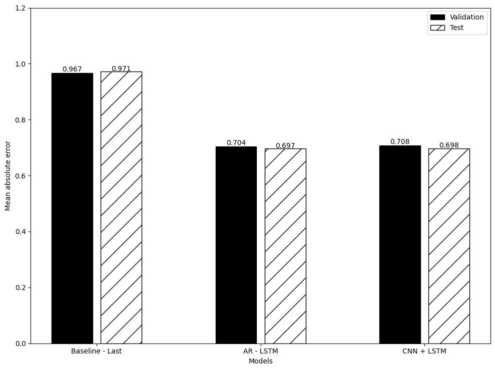
したがって今後、弊研究所の提供するPrometheusシリーズについても「ARLSTM」すなわち自己回帰型モデルの採用を検討すべきであるという方向性が今回の実験によって示すことが出来たと考える。MAEを用いた実に僅差の結果ではあるが、結果は結果である。引き続きPrometheus I/IIを超えるモデル構築を目指して、精進していくこととしたい。
2024年2月11日 東京・丸の内にて
株式会社原田武夫国際戦略情報研究所 代表取締役・CEO/グローバルAIストラテジスト
原田 武夫記す
(参考文献)
[Peixeiro 23] Peixeiro, Marco: Pythonによる時系列予測, マイナビ出版, 2023